This goes out to my Calculus class. Enjoy! 🙂

This goes out to my Calculus class. Enjoy! 🙂
I’m currently taking a grad class in differential equations. I just had a homework problem that asked about the heat conduction in a long, thin rod. It inspired me to create another GeoGebra applet, and I thought I’d share. The math might be a bit inaccessible, but the results are fairly straightforward.

Consider a solid rod of some kind of uniform material (maybe aluminum or cast iron). Say it’s 20 cm long. And say, for whatever reason, the temperature at a given place in the bar is initially given by this distribution:

Notice the bar is 70 degrees at each end and 50 degrees in the middle. (This is arbitrary…I just picked this distribution, just for fun.)
Now, let’s say the sides of the bar are insulated, and we just apply heat to the ends. If we maintain a temperature of 10 degrees at one end and 50 degrees at the other end, after a long time, we would expect the temperature throughout the bar to be evenly distributed, ranging from 10 degrees to 50 degrees. It would look something like this:
Now, the question is, what is the temperature throughout the bar after 1 second? It should be pretty close to the original distribution still, right? Right. What about after 10 seconds? 30 seconds? 30 days? Eventually it will look like the above distribution. That’s why we call this the “steady-state” distribution.
Here’s what the temperature throughout the bar looks like after 30 seconds, for instance.

Notice that the temperature distribution is still very similar to the initial distribution, but that the ends are changing temperature. This will happen more and more over time.
The applet I constructed lets you change everything about this situation: the length of the bar, the type of material, the temperature we apply to each end, and the initial temperature distribution. Like I said, the math is a bit nasty, but the results are intuitive, I hope. If you want to see some more of the math, feel free to do some reading!

My Precalculus students have been asking me this question. I don’t really have a great answer, except that it’s true. Granted it’s not very intuitive. But nothing about infinite series is intuitive. For those not in my class or not familiar with the harmonic series, the question is:
Does 
And the answer is no. This is surprising, because the terms of the series approach zero.
The proof that it diverges is due to Nicole Oresme and is fairly simple. It can be found here. There are at least 20 proofs of the fact, according to this article by Kifowit and Stamps.
Interestingly, the alternating harmonic series does converge:
And so does the p-harmonic series with p>1. For instance:
Besides looking at the sequence of partial sums, I’m not sure I can help you with the intuition on any of these facts. Can you?
Check out this TED talk. It’s very good, and relatively short.
Comments?
I posted this problem a few weeks ago:
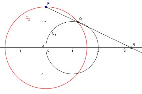
The figure shows a fixed circle 


And I also posted this applet, so you could investigate it yourself.
Now, I post the solution. Initially, I thought that the 
Remembering that 
Now, we seek to find the coordinates of 
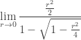
We now take the limit of 
If we try to evaluate this limit by plugging in 0, we get an indeterminant form 0/0. We can either use L’hopital’s Rule or evaluate it numerically. Either way, we find.
I have to say, this result surprised me. Like I said, I expected this limit to evaluate to 0 or infinity–but 4?? I had to get a bit more of an intuitive understanding, so I built that Geogebra applet.
Also, I was told afterward, by the student who brought this to me, that there’s a straight-forward geometric way of deriving the answer, based on the observation that point Q and point R and the point (2,0) (0,2) form an isosceles triangle for all values of r. The observation isn’t trivial. Can you prove it’s true? Once you do realize this fact, though, the above result is clear.
I just posted this problem the other day.

I made this java applet to help visualize the problem. Give it a try. Use the slider to let r go to zero and see where point R goes. You’re sure to figure it out just by playing with the diagram. Now, can you prove it?
Here are a few recent things I’ve come across I thought everyone might enjoy:
Okay, I think you’re all caught up on the math world :-).
Here’s a great problem that a student brought to me today. For those who’ve been wanting a ‘problem of the month,’ here you go:
The figure shows a fixed circle
NPR’s Science Friday had an episode highlighting the mathematics behind the Saint Louis Arch. You can watch a little video on the subject at their website, here.
The shape of the arch is the same shape of a hanging chain, called a catenary. “Catenary” is another name for the hyperbolic cosine function,
It’s not the world’s most riveting video, but it does highlight this important function that doesn’t get much press in our high school math curriculum. If you watch the video, you’ll learn something about this function, and you’ll learn that the catenary is not only the shape of a hanging chain but also the shape of the most stable arch. For more on the mathematics of the Saint Louis Arch, visit the wikipedia article.
In particular, the Saint Louis Arch has the equation
Now, of course you want to know about the hyperbolic sine function, too. I’ll let you look it up yourself (or maybe you can take a guess, first?). Then ask yourself some questions you might be dying to know: Which functions are odd/even? What trig identities are associated with these functions? For Calculus students: What is the derivative of each of these functions? What is the power series? And there are some exciting connections with these functions and complex numbers, too. Go play, and tell me what you learn!
In our IB Precalculus class, we are in the middle of our Vectors and Parametric Equations unit. It’s one of my favorites. And it just so happens that Dave Richeson just created some fantastic java applets with Geogebra that let users play around with properties of vectors. He blogged about it today, here. All of you should go check it out.

Thanks, Dr. Richeson!


