Disclaimer
Within my small inner circle of math teachers, the mystery of extraneous solutions seems to be the issue of the year. I have so much to say on this topic (algebraic, logical, pedagogical, historical, linguistic) that I don’t really know where to begin. My only disclaimer is that I’m not really sure if this topic is all that important.
Solving an Equation with a Radical Expression
Consider the following equation:
(1) 
One hardly needs algebra skills or prior knowledge to solve this, but prior experience suggests trying to isolate  .
.
(2)  (we subtract 5 from both sides)
(3)  (we divide both sides by 2)
Now, if the square root of something is 3, then that something must be 9, so it immediately follows that
(4) 
(5)  (we subtract 8 from both sides)
Squaring Both Sides
In my transition from (3) to (4), I used a bit of reasoning. Some conversational common sense told me that “if the square root of something is 3, then that something must be 9”. But that logic is usually just reduced to an algebraic procedure: “squaring both sides”. If we square both sides of equation (3), we get equation (4).
On the one hand, this seems like a natural move. Since the meaning of  is “the (positive) quantity which when squared is
  “, the expression is practically begging us to square it. Only then can we recover what lies inside. A quantity “which when squared is ” is like a genie “which when summoned will grant three wishes”. In both cases you know exactly what to do next.
Unfortunately, squaring both sides of an equation is problematic. If  is true, then
  is also true. But the converse does not hold. If , we cannot conclude that , because opposites have the same square.
This leads to problems when solving an equation if one squares both sides indiscriminately.
A Silly Equation Leads to Extraneous Solutions
Consider the equation,
(6) 
This is an equation with one free variable. It’s a statement, but it’s a statement whose truth is impossible to determine. So it’s not quite a proposition. Logicians would call it a predicate. Linguistically, it’s comparable to a sentence with an unresolved anaphor. If someone begins a conversation with the sentence “He is 4 years old”, then without context we can’t process it. Depending on who “he” refers to, the sentence may be true or false. The goal of solving an equation is to find the solution set, the set of all values for the free variable(s) which make the sentence true.
Equation (6) is only true if has value 4. So the solution set is  . But if we square both sides for some reason…
(7)  has solution set
We began with , “did some algebra”, and ended up with . By inspection,  is a solution to , but not to the original equation which we were solving, so we call an “extraneous solution”. [Extraneous – irrelevant or unrelated to the subject being dealt with]
Note that the appearance of the extraneous solution in the algebra of (6)-(7) did not involve the square root operation at all. But this example was also a bit silly because no one would square both sides when presented with equation (6), so let’s look at a slightly less silly example.
Another Radical Equation
(8) 
(9) 
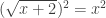
(10) 
People paying attention might stop here and conclude (correctly) that (10) has no solutions, since the square root of a number can not be negative. Closer inspection of the logic of the algebraic operations in (8)-(10) enables us to conclude that the original equation (8) has no solutions either. Since  , any solution to (8) will also be a solution to (9) and vice versa. Since
  , any solution to (9) will also be a solution to (10) and vice versa. So equations (8), (9), and (10) are all “equivalent” in the sense that they have the same solution set.
But what if the equation solver does not notice this fact about (10) and decides to square both sides to get at that information hidden inside the square root?
(11)
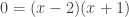
(12)
Again we have an extraneous solution. is a solution to (12), but not to the original equation (8). Where did everything go wrong? By the previous logic, (8), (9), and (10) are all equivalent. (11) and (12) are also equivalent. So the extraneous solution somehow arose in the transition from (10) to (11), by squaring both sides.
So unlike subtracting 5 from both sides or dividing both sides by 2, squaring both sides is not an equivalence-preserving operation. But we tolerate this operation because the implication goes in the direction that matters. If , then , so if and  are expressions containing a free variable , any value of that makes true will also make true.
In other words, squaring both sides can only enlarge the solution set. So if one is vigilant when squaring both sides to the possible creation of extraneous solutions, and is willing to test solutions to the terminal equation back into the original equation, the process of squaring both sides is innocent and unproblematic.
Those Who are Still Not Satisfied
Still there are some who are not satisfied with this explanation: “Why does this happen? What is really going on? Where do the extraneous solutions come from? What do they mean?”
One source of the problem is the square root operation itself. is, by the conventional definition, the positive quantity which when squared is . The reason that we have to stress the positive quantity is that there are always two real numbers that when squared equal any given positive real number. There are a few slightly different ways of making this same point. The operation of squaring a number erases the evidence of whether that number was positive or negative, so information is lost and we are not able to reverse the squaring process.
We can also phrase the phenomenon in the language of functions. Since squaring is a common and useful mathematical practice, information will often come to us squared and we’ll need an un-squaring process to unpack that information.  , for all the reasons just mentioned, is not a one-to-one function, so strictly speaking, it is not invertible. But un-squaring is too important, so we persevere. As with all non-one-to-one functions, we first restrict the domain of to
  to make it one-to-one. This inverse,
  thus has a positive range and so the convention that
  is born. So every use of the square root symbol comes with the proviso that we mean the positive root, not the negative root. We inevitably lose track of this information when squaring both sides.
[Note: Students can easily lose track of these conventions. After a lot of practice solving quadratic equations, moving from  effortlessly to
  , students will often start to report that
  .]
.]
The convention that we choose the positive root is totally arbitrary. In a world in which we restricted the domain of to ![(-\infty, 0]](https://s0.wp.com/latex.php?latex=%28-%5Cinfty%2C+0%5D&bg=ffffff&fg=333333&s=0&c=20201002) before inverting,
before inverting,  would be
  . In that world, is a perfectly good solution to , not extraneous at all.
A Trigonometric Equation which Yields an Extraneous Solution
For parallelism, consider the (somewhat artificial) equation:
(13) 
Like in (10), careful and observant solvers might notice that the range of the  function is
 ![[0, \pi]](https://s0.wp.com/latex.php?latex=%5B0%2C+%5Cpi%5D&bg=ffffff&fg=333333&s=0&c=20201002) and correctly conclude that the equation has no solutions. But there seems to be a lot going on inside that
and correctly conclude that the equation has no solutions. But there seems to be a lot going on inside that  expression, so many will rush ahead and try to unpack it by “cosineing”. Indeed, since
  , this seems innocent.
(14) 
(15) 
(16) 
But is an extraneous solution since  not
not  .
.
The explanation for this extraneous solution will be similar to the logic we used above. If , then  , so if and are expressions containing a free variable , any value of that makes true will also make true. So we will not lose any solutions by “taking the cosine of both sides”. But as the cosine function is not one-to-one, does not imply that . So taking the cosine of both sides, just like squaring both sides, can enlarge the solution set.
The above paragraph explains why extraneous solutions could appear in the solution of (13), but maybe not why they do appear. For that, we again must look to the presence of the function. Since  is not one-to-one, we had to arbitrarily restrict its domain to prior to inverting. So every use of the symbol comes with its own proviso that we are referring to a number in a particular interval of values. In a world in which we had restricted the domain of to
 ![[\pi, 2\pi]](https://s0.wp.com/latex.php?latex=%5B%5Cpi%2C+2%5Cpi%5D&bg=ffffff&fg=333333&s=0&c=20201002) prior to inverting, would be a perfectly good solution to , not extraneous at all.
prior to inverting, would be a perfectly good solution to , not extraneous at all.
The above examples seem to suggest that one can avoid dealing with extraneous solutions by carefully examining one’s equations at each step. But in practice, this really isn’t possible. I saved the fun examples for the end, but as this post is already way way too long, they will have to wait for a bit later.
-Will Rose
Thanks
Thanks to John Chase for letting me guest post on his blog. Thanks to James Key for encouraging me again and again to think about extraneous solutions.


 ____________________________________________________________________________________


 :
:

 :
:


 , you obtain the following result from arithmetic:
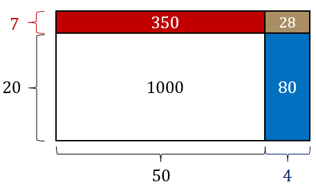
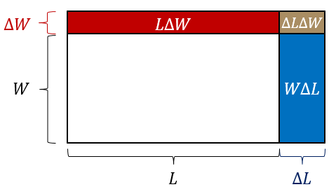
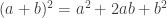
 can be thought of as the change in the area of a rectangle with side lengths
  and
and  . That is, let
  . As we change
  and
and  , we are wondering how the overall area changes (that is, what is
  ?).
?). . Similarly, the width is now
  . It follows that the new area is:

 gives:
 gives the desired result:
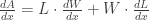


 for any well-defined function
  . If
. If  so any solution of
  and
and  in that order. Since all three of the functions are one-to-one, we are assured that (1) and (4) are equivalent. If we had cause to apply a non-one-to-one function, then we should be vigilant for extraneous solution.

 We squared!
 We squared again!


 , we should be vigilant for extraneous solutions. [Note: since both sides of (6) are necessarily positive, applying
  is not. I am more or less content to leave it at that. But some may ask for more clarity as to exactly what happened and when, so let’s indulge them.


 is created and it appears exactly where we would expect it, in the transition from (8) to (9) as we replaced (8) with the result of applying the non-one-to-one function
  , which is false, but (9) reads
  , which is true. For this particular value of
  is not a solution to (8) or to any previous equation in the solving sequence, but is a solution to (9) and thus to all subsequent equations in the solving sequence.
 , it does not surprise us that,
 .
.


 , we don’t mean
  . Take, for example, the following algebra which results in an extraneous solution:


 ). Here the last line doesn’t hold because only one solution satisfies the original equation (
 ). Remember that our logic is still flawless, though. Our logic just says that IF
  in order to prove statement A is true from premise C. The argument begs the question.
 ” is the missing logical connection.
 with lower bound
  .
. and
and  . (definitions of lower and upper bound)
 for
for  , I would expect this kind of work for “full credit”:


 as justification for conclusion A from premise C, but I would want a student to say “A is true if and only if B is true, which is true if and only if C is true.” Even though it provides a valid proof, I discourage students from using this somewhat cumbersome construction.


 ?
? or
or
 but what about
  aka.
aka. 
-\frac{1}{8}\left(\frac{a}{b}\right)^2+\frac{1}{16}\left(\frac{a}{b}\right)^3+\cdots\right)")

