At some point in every calculus class, we must discover and prove the product rule for derivatives. How a calculus teacher chooses to do this probably says a lot about their pedagogy and educational priorities.
Some teachers might simply write the rule on the board, expect students to accept it, and immediately launch into examples. Should we try to let the students discover the formula on their own? Should we perhaps lead them into a trap by suggesting that the derivative of a product of two functions is the product of the derivatives and let them find counterexamples? Should we state the theorem, but let the students try to prove it on their own? Should we perhaps have an entire mini-lesson on what it even means to have a product of two functions?
Should we try to motivate the entire discussion with a particularly intuitive pair of functions whose product has some real-world significance? Should we interpret the product of two functions geometrically, as the area of the corresponding rectangle? If properly motivated and explained, do we actually gain anything by doing the rigorous proof via limits?
The Status Quo
As a foil, here is the introduction to and proof of the product rule from the textbook that I teach out of.

I understand that textbooks have limited space and are no substitute for a full curriculum, but I think we can all agree that this is awful. There is no motivating example and no geometric intuition is called upon. The author merely proves the theorem, dryly and without understanding or purpose. The author even admits that the proof is unsatisfying and unedifying and apologizes in advance for its opaque maneuvers! Some proofs involve “clever steps that may appear unmotivated to a reader”.
In other words, reader, I am clever and you are not. This proof crucially involves cleverness, but since you’re not clever, you never would have thought of it yourself. I will perform some algebraic manipulations here in blue — they may appear unmotivated to you, but that’s your fault. In fact, I haven’t motivated them at all, but I don’t need to explain my clever methods to you. This is a calculus textbook after all, not a motivational textbook on explaining one’s cleverness. I have proved the rule, what else do you want me to do? If you want meaning and understanding, please consult your local religious figures for guidance.
Can we do better? Yes, I think we can. My friend James Key and I have used the phrase “tyranny of the blue text” to refer to totally opaque and unmotivated algebraic moves in textbook math proofs, since the offending expressions are often rendered in blue. Proving an important theorem to students via seemingly arbitrary, unmotivated algebraic tricks is an intellectual crime, and we should endeavor to banish the tyranny of the blue text from our classrooms and from our consciousness.
Idea #1: A Word Problem
Suppose a particular factory produces toys 24 hours a day.
Let  be a continuous model of the number of workers at the factory at time
  . The value of this function fluctuates throughout the day as workers leave and arrive according to their various particular schedules.
Let  be a continuous model of the number of toys produced per worker per hour at time . This function measures the overall efficiency of the factory at a particular time of day. This could reasonably be expected to fluctuate due to external factors like the electricity supply, the weather (solar panels!), or the tiredness of the workers.
Then  is the total rate at which the factory produces toys, measured in toys per hour, at a particular time .
 is the rate of change of
  with respect to , in other words the rate at which the workforce at the factory is rising or falling, as workers leave and arrive.
 is the rate of change of
  with respect to , in other words the rate at which the efficiency of the factory (on a per worker basis) is changing at a particular time .
 is the rate at which the factory’s output is changing, at a given time . In other words, if is positive and big, the factory’s output is increasing a lot at that moment, but if is positive and small, the factory’s output is increasing only a little at that time .
Using our own common sense, what should depend on? Surely is relevant, since even if efficiency holds steady, if workers are pouring into the factory at time , the factory’s output will go up. But surely is also relevant, since even if the workforce holds steady, if the workers are becoming more efficient, then the factory’s overall output will go up. But the current size of the workforce, , is also relevant, since if, for example, efficiency is going up but the current workforce is very small, those gains in efficiency will not translate into large increases in output. And the current efficiency, , is also relevant, since if, for example, workers are pouring into the factory, but the current toy production per worker per hour is very small, then those extra workers will also not translate into large increases in output.
Just by having these conversations, we prime our students to have a deep appreciation of what the product rule is about, what differentiation is about, why we would ever want to multiply two functions, and why we would ever want to learn calculus.
This year, when giving this exact introduction to the product rule, I had a student guess the product rule right there on the spot, just from talking out the logic of the toy factory.
Idea #2: A Geometric Interpretation
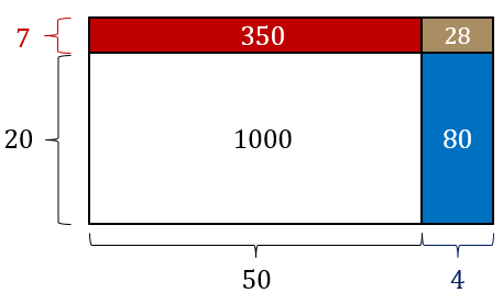
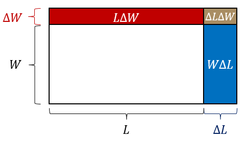
Some calculus textbooks motivate the product rule geometrically, by interpreting the product of two functions as the area of the rectangle whose side lengths are the values of the two functions at a given time.

This sloppy picture is taken from a presentation I gave at an NCTM conference a few years ago about calculus proofs. The area of the rectangle with side lengths  and
and  represents the value of the
  function at a particular time. A moment later, both and change, and the derivative wants to measure the size of the change. Here again, we can read the product rule directly off the diagram. A “proof” like this was probably totally sufficient to a mathematician of the 18th century, but in a post-Cauchy/Weierstrass world, we need to verify these intuitions via the definition of the derivative as a limit.
But we can hold onto our geometric intuition and have our rigor as well!

The same diagram can be used to interpret that mysterious numerator in the definition of the derivative and avoid the tyranny of the blue text. The diagram motivates, but the rigor is preserved, since the limit just under the rectangle can be expanded and verified to be equivalent to the limit just above the diagram. But this time we are doing the proof with meaning and understanding.
Teaching the product rule this way might even be considered “standard”. The only drawback is that you do kind of have to be clever to think to do all this! Would a student come up with the idea to make a rectangle on their own? I’m not sure. I don’t claim to be the first or the only one to use a rectangle to discover, motivate, and even prove the product rule, but the following is something I have never seen anywhere before and that I just came up with a month ago. It is the excuse to write this blog post.
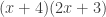
Idea #3: Start with a particular example

I’m getting a bit tired, so I pasted this picture in. The idea is simple. Combine a function with a known derivative and a generic second function . And then just try to find the derivative of the product. No understanding or geometric intuition is required, but no teacher help or input is probably required either.
A reasonable calculus student who is confident, good at algebra, and experienced with limits and computing derivatives from the definition should be able to get to the end by just doing what comes natural.
I have not tried this before in class, so I can’t say how well it will work. But if it works, then the students have proved themselves to be every bit as clever as is required, and they’ve done it on their own. The teacher can then add extra layers of understanding to the general phenomenon of the product rule and lead the class through the general proof, possibly using geometry as a guide. But the students who figured out this particular example will feel that they could have done the general case on their own. And they will be right.


 ____________________________________________________________________________________


 :
:

 :
:


 , you obtain the following result from arithmetic:
 can be thought of as the change in the area of a rectangle with side lengths
  and
and  . As we change
  and
and  , we are wondering how the overall area changes (that is, what is
  ?).
?). . Similarly, the width is now
  . It follows that the new area is:

 gives:
 gives the desired result:
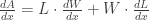


 , which has an unambiguous inflection point at
  .
. we have
  and for
  we have
  , or vice versa.*
 . That is,
  does not have a point of inflection at
  , the definition of the function is no longer at issue. Yet we would all agree that
  does not constitute a point of inflection, right? The continuity requirement seems to formalize our intuition here.
![f(x)=\sqrt[3]{x}](https://s0.wp.com/latex.php?latex=f%28x%29%3D%5Csqrt%5B3%5D%7Bx%7D&bg=ffffff&fg=333333&s=0&c=20201002) . Here we have a concavity change (concave up to concave down) across
. Here we have a concavity change (concave up to concave down) across  is undefined.
 shown above has a point of inflection at


![\int_{-1}^1 \frac{1}{x}dx = \lim_{a\to 0^+}\left[\int_{-1}^{-a}\frac{1}{x}dx+\int_a^{1}\frac{1}{x}dx\right]](https://s0.wp.com/latex.php?latex=%5Cint_%7B-1%7D%5E1+%5Cfrac%7B1%7D%7Bx%7Ddx+%3D+%5Clim_%7Ba%5Cto+0%5E%2B%7D%5Cleft%5B%5Cint_%7B-1%7D%5E%7B-a%7D%5Cfrac%7B1%7D%7Bx%7Ddx%2B%5Cint_a%5E%7B1%7D%5Cfrac%7B1%7D%7Bx%7Ddx%5Cright%5D&bg=ffffff&fg=333333&s=0&c=20201002)
![= \lim_{a\to 0^+}\left[\ln(a)-\ln(a)\right]=\boxed{0}](https://s0.wp.com/latex.php?latex=%3D+%5Clim_%7Ba%5Cto+0%5E%2B%7D%5Cleft%5B%5Cln%28a%29-%5Cln%28a%29%5Cright%5D%3D%5Cboxed%7B0%7D&bg=ffffff&fg=333333&s=0&c=20201002)
![\int_{-1}^1 \frac{1}{x}dx = \lim_{a\to 0^+}\left[\int_{-1}^{-a}\frac{1}{x}dx+\int_{2a}^{1}\frac{1}{x}dx\right]](https://s0.wp.com/latex.php?latex=%5Cint_%7B-1%7D%5E1+%5Cfrac%7B1%7D%7Bx%7Ddx+%3D+%5Clim_%7Ba%5Cto+0%5E%2B%7D%5Cleft%5B%5Cint_%7B-1%7D%5E%7B-a%7D%5Cfrac%7B1%7D%7Bx%7Ddx%2B%5Cint_%7B2a%7D%5E%7B1%7D%5Cfrac%7B1%7D%7Bx%7Ddx%5Cright%5D&bg=ffffff&fg=333333&s=0&c=20201002)
![= \lim_{a\to 0^+}\left[\ln(a)-\ln(2a)\right]=\boxed{\ln{\frac{1}{2}}}](https://s0.wp.com/latex.php?latex=%3D+%5Clim_%7Ba%5Cto+0%5E%2B%7D%5Cleft%5B%5Cln%28a%29-%5Cln%282a%29%5Cright%5D%3D%5Cboxed%7B%5Cln%7B%5Cfrac%7B1%7D%7B2%7D%7D%7D&bg=ffffff&fg=333333&s=0&c=20201002)
![\int_{-1}^1 \frac{1}{x}dx = \lim_{a\to 0^-}\left[\int_{-1}^{a}\frac{1}{x}dx\right]+\lim_{b\to 0^+}\left[\int_b^{1}\frac{1}{x}dx\right]](https://s0.wp.com/latex.php?latex=%5Cint_%7B-1%7D%5E1+%5Cfrac%7B1%7D%7Bx%7Ddx+%3D+%5Clim_%7Ba%5Cto+0%5E-%7D%5Cleft%5B%5Cint_%7B-1%7D%5E%7Ba%7D%5Cfrac%7B1%7D%7Bx%7Ddx%5Cright%5D%2B%5Clim_%7Bb%5Cto+0%5E%2B%7D%5Cleft%5B%5Cint_b%5E%7B1%7D%5Cfrac%7B1%7D%7Bx%7Ddx%5Cright%5D&bg=ffffff&fg=333333&s=0&c=20201002)
![= \lim_{a\to 0^-}\left[\ln|a|\right]+\lim_{b\to 0^+}\left[-\ln|b|\right]](https://s0.wp.com/latex.php?latex=%3D+%5Clim_%7Ba%5Cto+0%5E-%7D%5Cleft%5B%5Cln%7Ca%7C%5Cright%5D%2B%5Clim_%7Bb%5Cto+0%5E%2B%7D%5Cleft%5B-%5Cln%7Cb%7C%5Cright%5D&bg=ffffff&fg=333333&s=0&c=20201002)
 and the second is
  and the overall expression has the indeterminate form
  . In our very first approach, we assumed the limit variables
  and
and  were the same. In the second approach, we let
  . But one assumption isn’t necessarily better than another. So we claim the integral diverges.
 . For goodness sake, it’s symmetric about the origin!
 between -1 and 1, and then throw darts at the graph uniformly, wouldn’t you bet on there being an equal number of darts to the left and right of the y-axis?
